
An artificial neural network (ANN), neural network, or neural network is a computational mathematical model, developed inspired by brain or cognitive processes that take place in a natural neural network and used as part of machine learning. This type of network usually contains a large number of information units (input and output) connected to each other, connections that often pass through “hidden” information units (Hidden Layer). The form of connection between the units, which contains information about the strength of the connection, simulates how the neurons in the brain connect. The use of artificial neural network is mainly common in the cognitive sciences, and in various software systems – including many artificial intelligence systems that perform a variety of tasks – character recognition, face recognition, handwriting recognition, capital market forecasting, speech recognition system, image recognition, text analysis and more.
A neural network is a network of linked processors:
Each processor in a network is capable of performing a simple mathematical operation. But when linked together they are capable of complex behavior.
In the brain, nerve cells or neurons are the cells that make up the nervous system. And there are about one hundred billion of them in the average person. Each of them evolved to be an electronic processor. The dendrites receive information from the outside world and form the input system of the neuron. When enough stimuli are received in the dendrites. The cell body produces an electrical signal. That travels along the axon to the dendrites of other cells or muscles and stimulates them. The more stimuli the neurons receive from the dendrites, the more electrical signals they produce in one second.
How a neuron processes information
The main difference between a biological neural network and an artificial neural network is that computers operate primarily in serial processing. Or with a small amount of parallel processing, while the brains of creatures operate in parallel processing. According to Church and Turing’s thesis, the model is equivalent to a Turing machine. (since any calculation that can be done by a parallel computer can also be done by a serial computer).
There are some other important differences between neural network in the brain and artificial network. The brain has a huge number of components (about 1011). Each of which is connected to many components (between 1,000 and 10,000 on average). Each of these components performs a fairly simple calculation, the nature of which is still not entirely clear, relatively slowly. (less than one kilohertz), based primarily on information it receives from its local connections. In artificial systems, the nerve cells are uniformly connected to each other, and they all perform the same computational action. Each connection is assigned some numerical weight. The output of each cell is a single numerical value, calculated as a result of the sum of the operations of the input cells and their relative weight.
It is also possible to divide the nerve cell networks into two different groups, with guided or non-guided learning. Guided networks, such as the Perceptron, use a guided learning algorithm, which means that the system needs to receive and output information during the learning phase. In contrast, non-guided networks, such as the Kohonen network, only require information to be received, without output. These systems organize the information received themselves, according to a similarity index.
History
1943 – The development of the science of neural networks
In 1943, two American researchers, Vern McLaughlin and Walter Pitts published an article. Which formed the basis for the development of neural network science. The article proposed a simple model of neuron action, on which artificial networks are based to this day:
An example of a basic artificial neuron. Four input data, marked with i1 to i4. These represent the dendrites and can be connected to the outside world or to other neurons. For a relative “weight” input, expressed by weights denoted by: w1 to w4. These weights represent the strength of the bonds between the dendrites of one neuron and the cell body in a second true neuron
The neuron receives inputs (usually marked with i), each of which has a relative weight (usually marked with a w). Each figure is weighed by multiplying it by the appropriate weight, with the result of the sum of the weighted inputs:
Sum =
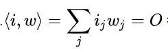
If this sum (which in the biological sense is the total stimulus due to the neuron) is higher than any known threshold the neuron transmits output “1”; If not, the output is “0”.
This process is reminiscent of the action of a real neuron. Which produces an electrical signal when the stimulus is sufficient.
Using a pattern recognition neuron. You can encode the dark pixels at 1 and the light pixels at 0. Now, if we connect our neuron as shown in Figure B, it will output “1” whenever it sees this pattern. Even if the pattern is not perfect – the ones are not exactly one, and the zeros are not exactly zero – the neuron will still recognize the pattern (in this case it is said that the neuron is soundproof). However, if we insert a completely different pattern like the one shown in Figure 6C, the neuron will not recognize it.
The arrangement of the weights is essential for the functioning of the network. The weights are the ones that determine what pattern will be identified, and determining them is the central task of the neural network program.
1969 – Abandonment of networks following an article on the limitations of neural networks
In 1969, Marvin Minsky and Seymour, and Papert published their book, Perceptrons, in which they attacked the ideas behind neural networks. The book presented a defect in the basal neuron.
The problem was this: no matter what women weights on the input, we could not create the Exclusive OR (XOR) logical gateway for a single-layer network. In addition, they argued that computers do not have enough computing power to handle complex networks. These and other arguments have delayed the continued development of neural networks for many years. Many researchers have abandoned the field in their minds because if the neuron cannot perform this simple task, there is no point in continuing the study.
In fact, what was needed to overcome this problem and similar problems is not a single neuron, but a network of neurons, and the Russian mathematician Andrei Kolmogorov has already shown that a network of neurons in 3 layers can solve XOR.
Multilayered neural network
1982 – The re-emergence of neural networks(Artificial neural network) in the 1980s
Although the solution was known, it was not until 1982–1983 that interest in neural network research resurfaced. During this time, the “backward slashing algorithm” gained widespread publicity.
The 2000s – Deep Learning
Artificial neural network have undergone a renaissance since the first decade of the 2000s. It was during this period that the term “deep belief nets” and the acronym for deep nets, which was coined in a 2006 influential article by Hinton, Osindro Veta, began to be popular. As part of deep learning, the use of artificial neural network with several hidden layers has become common.
During this period, the interest of commercial companies in artificial neural network increased. Since 2012, all winners of major computer vision competitions in the field of object recognition, such as the ImageNet competition, are based on deep learning.
Naturally, after in 2012, “deep learning” was the “algorithm” that won the ImageNet competition, and the network architectures received a lot of attention, both in academia and industry.
Neural network Structure
A neural network consists of a large number of base cells, so each base cell performs a relatively simple calculation. Each cell has several inputs and one output its value is some function of the inputs. An output of a particular cell can enter multiple inputs of different cells.
There are many models of neural networks(Artificial neural network). What they all have in common is the existence of solitary processing units (equivalent in the model to biological neurons) that are interconnected (similar to the existing relationships between biological neurons). The details – the number of neurons, the number of connections, the structure of the network (arrangement in layers, the number of layers) – vary from model to model. It is common to use tools from the field of linear algebra such as vector matrices to represent the neurons and the connections between them. The action performed by each neuron on its input is usually represented by a function.
A neural network is characterized by:
- Connections – how to connect the neurons in the network
- Weights – The method that determines the weights of connections between neurons
- The activation function may be different in each layer (non-linear function, usually sigmoid)
Neuron networks consist of a large number of simple processing units called neurons, which are hierarchically connected and layered. The first layer is intended to receive information to the network, the middle layer is known as the hidden layer (in different models there may be more than one such), and finally, the last layer which is intended to return the processed information as output.
The nodes in each layer are fully connected to the nodes in the adjacent layers through a direct connection between the neurons, with each knot having a certain weight. The weight of each connection determines how relevant the information passing through it is, and whether the network should use it to solve the problem. Each node in the input layer (the first layer) represents a feature different from the structure, and the output layer represents the solution to the problem. In the middle and outer layer, there are “threshold values” that can be calibrated in a computerized system, and determine the importance of the various relationships,
There are 3 types of layers in the network:
Input Layer – Each cell in this layer has one input. The input vector is the input to the network. The number of cells: As the number of features. It is advisable to conduct research regarding the effect of the various characteristics on the error, relationships, and hierarchy between them. A rule of thumb is that the total number of characteristics should not exceed one-tenth of the number of examples in the study series.
Hidden Layers – Each cell in this layer has a number of inputs, as the number of entry cells (Fully Connected). A network of neurons without hidden layers is very limited and is called a perceptor. The number of cells: As the number of cells in the entry layer plus one or two cells. The number of layers: from 0 to infinity. In all the hidden layers usually the same number of cells. It is advisable to conduct research regarding the effect of the number of cells and the number of hidden layers on the error.
The number of layers and the number of cells define the size of the network. Choose a network large enough, but not too large. A network that is too small will not be able to bring the required mapping close enough. While a network that is too large will prevent effective learning (this is the Bias Trade-Off). Typical multilayer networks have one or two hidden layers. And the number of neurons in the hidden layers often does not exceed 10 (unless there is a modular division into a number of sub-networks). Image recognition problems are usually characterized by a very high number of layers (hundreds of layers). Adjustment of the number of neurons and the structure of the network will usually be done empirically. Using validation examples or through cross-validation.
Output Layer – Each cell in this layer has a number of inputs. As the number of cells in the hidden layer (Fully Connected). The cell output vector in this layer is the network output vector. The number of cells: As the number of classes.
Activation function
Some of the features that may be useful for an activation function:
- Nonlinear – When the function is not linear, a two-layered neural network(Artificial neural network) can be shown to be of universal value. The identity function does not maintain this feature. When multiple layers use ID function activation, the network is equivalent to a single-layer model.
- Continuous Shear – This is a desirable feature that aids in gradient-based optimization. A binary degree function is not differentiable at 0. And its derivative is 0 for other values, so gradient-based methods may get stuck.
- Range – When the range of the activation function is final, gradient-based training methods tend to be more stable. Because the representation of the pattern is greatly affected by limited weights. When the range is infinite, the training is usually more effective as representing patterns affects most of the weights.
- Monotonic – When the activation function is monotonic, the error area associated with a single-layer model is guaranteed to be convex.
- Often detected near the main point – when the activation function is endowed with this feature. The network learns efficiently when the weights are initialized to small random values. When this feature does not exist in the activation function, attention is required in initializing the weight values.